Reward Modeling
Reward models are core to the modern approach to RLHF by being where the complex human preferences are learned. They are what enable our models to learn from hard-to-specify signals. They compress complex features in the data into a representation that can be used in downstream training – a sort of magic that once again shows the complex capacity of modern deep learning. These models act as proxy objectives for the core optimization, as studied in the following chapters. As shown in fig:rm-role-in-rlhf?, the reward model plays a role like the standard RL environment, providing the learning signal for the agent, but unlike a fixed environment, we get to learn it from human preferences.
Reward models have historically been used extensively in reinforcement learning research as a proxy for environment rewards [1]. Reward models were proposed, in their modern form, as a tool for studying the value alignment problem [2]. These models tend to take in some sort of input and output a single scalar value of reward. This reward can take multiple forms – in traditional RL problems it was attempting to approximate the exact environment reward for the problem, but we will see in RLHF that reward models actually output a probability of a certain input being “of high quality” (i.e. the chosen answer among a pairwise preference relation). The practice of reward modeling for RLHF is closely related to inverse reinforcement learning, where the problem is to approximate an agent’s reward function given trajectories of behavior [3], and other areas of deep reinforcement learning. The high-level problem statement is the same, but the implementation and focus areas are entirely different, so they’re often considered as totally separate areas of study.
The most common reward model, often called a Bradley-Terry reward model and the primary focus of this chapter, predicts the probability that a piece of text was close to a “preferred” piece of text from the training comparisons. Later in this section we also compare these to Outcome Reward Models (ORMs), Process Reward Models (PRMs), and other types of reward models.
Throughout this chapter, we use \(x\) to denote prompts and \(y\) to denote completions. This notation is common in the language model literature, where methods operate on full prompt-completion pairs rather than individual tokens.

Training a Bradley-Terry Reward Model
The canonical implementation of a reward model is derived from the Bradley-Terry model of preference [4]. There are two popular expressions for how to train a standard reward model for RLHF – they are mathematically equivalent. To start, a Bradley-Terry model of preferences defines the probability that, in a pairwise comparison between two items \(i\) and \(j\), a judge prefers \(i\) over \(j\):
\[P(i > j) = \frac{p_i}{p_i + p_j}.\] {#eq:bradterry}
The Bradley-Terry model assumes that each item has a latent strength \(p_i > 0\), and that observed preferences are a noisy reflection of these underlying strengths. It is common to reparametrize the Bradley-Terry model with unbounded scores, where \(p_i = e^{r_i}\), which results in the following form:
\[P(i > j) = \frac{e^{r_i}}{e^{r_i} + e^{r_j}} = \sigma(r_i-r_j).\] {#eq:bradterry_unbounded}
Here \(\sigma(z) = \frac{1}{1 + e^{-z}}\) is the logistic (sigmoid) function, so the preference probability depends only on the score difference \(r_i - r_j\). Only differences in scores matter: adding the same constant \(c\) to every \(r_k\) leaves \(P(i > j)\) unchanged. These forms are a useful approximation of human preferences that often works well in RLHF.
To train a reward model, we must formulate a loss function that satisfies the above relation. In practice, this is done by converting a language model into a model that outputs a scalar score, often via a small linear head that produces a single reward value from the model’s final hidden state. Given a prompt \(x\) and two sampled completions \(y_1\) and \(y_2\), we score both with a reward model \(r_\theta\) and write the conditional scores as \(r_\theta(y_i \mid x)\).
The probability that the reward model assigns to \(y_1\) being preferred to \(y_2\) becomes:
\[P(y_1 > y_2 \mid x) = \frac{\exp\left(r_\theta(y_1 \mid x)\right)}{\exp\left(r_\theta(y_1 \mid x)\right) + \exp\left(r_\theta(y_2 \mid x)\right)}.\] {#eq:bradterryrm}
We denote the preferred completion as \(y_c\) (chosen) and the rejected completion as \(y_r\).
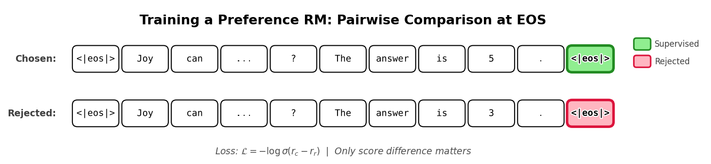
The resulting loss encourages the reward model to assign a higher score to the human-preferred completion than the rejected one, using a sigmoid to convert the score difference into a probability. The preference likelihood in eq:bradterryrm? is the starting point. We first rewrite that likelihood into sigmoid form by dividing the numerator and denominator by \(\exp\left(r_\theta(y_c \mid x)\right)\):
\[ \begin{aligned} P(y_c > y_r \mid x) &= \frac{\exp\left(r_\theta(y_c \mid x)\right)}{\exp\left(r_\theta(y_c \mid x)\right) + \exp\left(r_\theta(y_r \mid x)\right)} \\ &= \frac{\exp\left(r_\theta(y_c \mid x)\right)}{\exp\left(r_\theta(y_c \mid x)\right)\left(1 + \frac{\exp\left(r_\theta(y_r \mid x)\right)}{\exp\left(r_\theta(y_c \mid x)\right)}\right)} \\ &= \frac{1}{1 + \frac{\exp\left(r_\theta(y_r \mid x)\right)}{\exp\left(r_\theta(y_c \mid x)\right)}} \\ &= \frac{1}{1 + \exp\left(-(r_\theta(y_c \mid x) - r_\theta(y_r \mid x))\right)} \\ &= \sigma \left( r_\theta(y_c \mid x) - r_\theta(y_r \mid x) \right). \end{aligned} \] {#eq:bradterryrm_sigmoid}
The reward model is then fit by maximum likelihood over the preference dataset \(D\), maximizing the expected log-likelihood of the observed preferences. Because the logarithm is monotonic, this is equivalent to minimizing the expected negative log-likelihood:
\[ \begin{aligned} \theta^* &= \arg\max_\theta \mathbb{E}_{(x, y_c, y_r) \sim D}\left[ \log P(y_c > y_r \mid x) \right] \\ &= \arg\min_\theta \mathbb{E}_{(x, y_c, y_r) \sim D}\left[ -\log \sigma \left( r_\theta(y_c \mid x) - r_\theta(y_r \mid x) \right) \right]. \end{aligned} \] {#eq:bradterryrm_deriv}
Taking the logarithm before averaging over the dataset is what makes the negative-log-likelihood loss the right objective: maximizing the expected probability \(\mathbb{E}[P]\) is not the same as maximizing the expected log-probability \(\mathbb{E}[\log P]\).
The per-example loss is the log-sigmoid expression inside the expectation above, as in [5] and other works: \[\mathcal{L}(\theta) = - \log \left( \sigma \left( r_{\theta}(y_c \mid x) - r_{\theta}(y_r \mid x) \right) \right)\] {#eq:rewardmodeling1}
The second is a mathematically equivalent form expressed using the softplus function \(\log(1+e^x)\), as in [6] and other works: \[\mathcal{L}(\theta) = \log \left( 1 + e^{r_{\theta}(y_r \mid x) - r_{\theta}(y_c \mid x)} \right)\] {#eq:rewardmodeling2}
These are equivalent by letting \(\Delta = r_{\theta}(y_c \mid x) - r_{\theta}(y_r \mid x)\) and using \(\sigma(\Delta) = \frac{1}{1 + e^{-\Delta}}\), which implies \(-\log\sigma(\Delta) = \log(1 + e^{-\Delta}) = \log\left(1 + e^{r_{\theta}(y_r \mid x) - r_{\theta}(y_c \mid x)}\right)\). They both appear in the RLHF literature.
The Default Reward Model Architecture
The most common way reward models are implemented is through an abstraction similar to Transformers’ AutoModelForSequenceClassification, which appends a small linear head to the language model and produces a scalar reward score for a prompt-completion pair at training or inference. At inference time, the model outputs the relative likelihood that the piece of text is chosen as a single logit from the model.
Other implementation options exist, such as just taking a linear layer directly from the final embeddings, but they are less common in open tooling.
Implementation Example
Implementing the reward modeling loss is quite simple. More of the implementation challenge is on setting up a separate data loader and inference pipeline. Given the correct dataloader with tokenized, chosen and rejected prompts with completions, the loss is implemented as:
import torch.nn as nn
# inputs_chosen / inputs_rejected include the prompt tokens x and the respective
# completion tokens (y_c or y_r) that the reward model scores jointly.
rewards_chosen = model(**inputs_chosen)
rewards_rejected = model(**inputs_rejected)

loss = -nn.functional.logsigmoid(rewards_chosen - rewards_rejected).mean()
As for the bigger picture, this is often within a causal language model (a model that generates tokens left-to-right, predicting each token conditioned on all previous ones) that has an additional head added (and learned with the above loss) that transitions from the final hidden state to the score of the inputs. The code takes in standard transformer inputs – input_ids (tokenized text) and attention_mask (which marks real tokens vs. padding) – and extracts the hidden state (the model’s internal representation of the input) at the last real token, which is then passed through a linear layer to produce a scalar reward. This model will have a structure as follows:
import torch
import torch.nn as nn
import torch.nn.functional as F

class BradleyTerryRewardModel(nn.Module):
    """
    Standard scalar reward model for Bradley-Terry preference learning.

    Usage (pairwise BT loss):
        rewards_chosen = model(**inputs_chosen)    # (batch,)
        rewards_rejected = model(**inputs_rejected)  # (batch,)
        loss = -F.logsigmoid(rewards_chosen - rewards_rejected).mean()
    """
    def __init__(self, base_lm):
        super().__init__()
        self.lm = base_lm  # e.g., AutoModelForCausalLM
        self.head = nn.Linear(self.lm.config.hidden_size, 1)

    def _sequence_rep(self, hidden, attention_mask):
        """
        Get a single vector per sequence to score.
        Default: last non-padding token (EOS token); if no mask, last token.
        hidden: (batch, seq_len, hidden_size)
        attention_mask: (batch, seq_len)
        """

        # Index of last non-pad token in each sequence
        # attention_mask is 1 for real tokens, 0 for padding
        lengths = attention_mask.sum(dim=1) - 1  # (batch,)
        batch_idx = torch.arange(hidden.size(0), device=hidden.device)
        return hidden[batch_idx, lengths]  # (batch, hidden_size)

    def forward(self, input_ids, attention_mask):
        """
        A forward pass designed to show inference structure of a standard reward model.
        To train one, this function will need to be modified to compute rewards from both
         chosen and rejected inputs, applying the loss above.
        """
        outputs = self.lm(
            input_ids=input_ids,
            attention_mask=attention_mask,
            output_hidden_states=True,
            return_dict=True,
        )
        # Final hidden states: (batch, seq_len, hidden_size)
        hidden = outputs.hidden_states[-1]

        # One scalar reward per sequence: (batch,)
        seq_repr = self._sequence_rep(hidden, attention_mask)
        rewards = self.head(seq_repr).squeeze(-1)

        return rewards
In this section and what follows, most of the implementation complexity for reward models (and much of post-training) is around constructing the data-loaders correctly and distributed learning systems. Note, when training reward models, the most common practice is to train for only 1 epoch to avoid overfitting.
Reward Model Variants
Reward modeling is a relatively under-explored area of RLHF. The traditional reward modeling loss has been modified in many popular works, but the modifications have not solidified into a single best practice.
Preference Margin Loss
In the case where annotators are providing either scores or rankings on a Likert Scale (a rating scale with ordered categories indicating magnitude of preference, e.g. 1–5), the magnitude of the relational quantities can be used in training. The most common practice is to binarize the data along the preference direction, reducing the mixed information of relative ratings or the strength of the ranking to just chosen and rejected completions. The additional information, such as the magnitude of the preference, has been used to improve model training, but it has not converged as a standard practice. Llama 2 proposes using the margin between two data points, \(m(y_c, y_r)\), to distinguish the magnitude of preference:
\[\mathcal{L}(\theta) = - \log \left( \sigma \left( r_{\theta}(y_c \mid x) - r_{\theta}(y_r \mid x) - m(y_c, y_r) \right) \right)\] {#eq:rewardmodelingmargin}
For example, each completion is often given a ranking from 1 to 5 in terms of quality. In the case where the chosen sample was assigned a score of 5 and rejected a score of 2, the margin \(m(y_c, y_r)= 5 - 2 = 3\). Other functions for computing margins can be explored.
Note that in Llama 3 the margin term was removed as the team observed diminishing improvements after scaling.
Balancing Multiple Comparisons Per Prompt
InstructGPT studies the impact of using \(K = 4\) to \(9\) completions per prompt to rank, producing \(\binom{K}{2}\) pairwise comparisons from each prompt [5]. Because these comparisons are highly correlated (they share the same prompt), shuffling them into the dataset naively causes the reward model to overfit. To address this, they weight the loss updates per comparison per prompt – without reweighting, prompts with more completions would contribute more total loss simply because they generate more pairs. In practice, all \(\binom{K}{2}\) comparisons from a single prompt are typically included in the same training batch and averaged together, so each prompt contributes one grouped update rather than appearing across many separate batches. This reduces overfitting to individual prompts and prevents prompts with more sampled completions from dominating the loss. The loss function becomes:
\[\mathcal{L}(\theta) = - \frac{1}{\binom{K}{2}} \mathbb{E}_{(x, y_c, y_r)\sim D} \log \left( \sigma \left( r_{\theta}(y_c \mid x) - r_{\theta}(y_r \mid x) \right) \right)\] {#eq:rewardmodelinginstructgpt}
K-Wise Loss Function
There are many other formulations that can create suitable models of human preferences for RLHF. One such example, used in the popular, early RLHF’d models Starling 7B and 34B [7], is a K-wise loss function based on the Plackett-Luce model [8].
Zhu et al. 2023 [9] formalize the setup as follows. With a prompt, or state, \(s^i\), \(K\) actions \((a_0^i, a_1^i, \cdots, a_{K-1}^i)\) are sampled from \(P(a_0,\cdots,a_{K-1}|s^i)\). Then, labelers rank the \(K\) actions by preference, producing a permutation \(\sigma^i: [K] \mapsto [K]\), where \(\sigma^i(0)\) is the most preferred action. This yields a Plackett-Luce probability over the complete ranking of all \(K\) items:
\[P(\sigma^i|s^i,a_0^i,a_1^i,\ldots,a_{K-1}^i) = \prod_{k=0}^{K-1} \frac{\exp(r_{\theta\star}(s^i,a_{\sigma^i(k)}^i))}{\sum_{j=k}^{K-1}\exp(r_{\theta\star}(s^i,a_{\sigma^i(j)}^i))}\] {#eq:kwise_rm}
When \(K = 2\), this reduces to the Bradley-Terry (BT) model for pairwise comparisons. Regardless, once trained, these models are used similarly to other reward models during RLHF training.
Outcome Reward Models
The majority of preference tuning for language models and other AI systems is done with the Bradley-Terry models discussed above. For reasoning-heavy tasks, one can use an Outcome Reward Model (ORM). The training data for an ORM is constructed in a similar manner to standard preference tuning. Here, we have a problem statement or prompt, \(x\) and two completions \(y_1\) and \(y_2\). The inductive bias used here is that one completion should be a correct solution to the problem and one incorrect, resulting in \((y_c,y_{ic})\).
The architecture of the models used is very similar to a standard reward model, with a linear layer appended to a model that can output a single logit (in the case of an RM) – with an ORM, the training objective that follows is slightly different [10]:
[We] train verifiers with a joint objective where the model learns to label a model completion as correct or incorrect, in addition to the original language modeling objective. Architecturally, this means our verifiers are language models, with a small scalar head that outputs predictions on a per-token basis. We implement this scalar head as a single bias parameter and single gain parameter that operate on the logits outputted by the language model’s final unembedding layer.
To translate, this is implemented as a language modeling head that can predict two classes per token (1 for correct, 0 for incorrect), rather than a classification head of a traditional RM that outputs one logit for the entire sequence. Formally, following [11] this is a per-token binary cross-entropy loss:
\[\mathcal{L}_{\text{CE}}(\theta) = -\mathbb{E}_{(s,r)\sim \mathcal{D}}\left[r\log p_\theta(s) + (1-r)\log(1-p_\theta(s))\right]\] {#eq:orm_loss}
where \(r \in \{0,1\}\) is a binary label where 1 applies to a correct answer to a given prompt and 0 applies to an incorrect answer, and \(p_\theta(s)\) is the scalar proportional to the predicted probability of correctness from the model being trained. In code, this outcome label is copied onto every completion token, while prompt tokens are masked with -100 so they do not contribute to the loss.
Implementing an outcome reward model (and other types, as we’ll see with the Process Reward Model) involves applying the cross-entropy loss per-token based on whether the completion is a correct sample. This is far closer to the language modeling loss, where it does not need the structured chosen-rejected nature of standard Bradley-Terry reward models. In the simplified ORM training setup below, we are not sampling new tokens or training an LLM on next-token prediction; we feed a fixed prompt-completion sequence through the backbone and train the ORM head to predict correctness labels.
The model structure could follow as:
import torch.nn as nn
import torch.nn.functional as F

class OutcomeRewardModel(nn.Module):
    def __init__(self, base_lm):
        super().__init__()
        self.lm = base_lm  # e.g., AutoModelForCausalLM
        self.head = nn.Linear(self.lm.config.hidden_size, 1)

    def forward(self, input_ids, attention_mask=None, labels=None):
        """
        input_ids contains a full prompt+completion sequence.
        labels is token-aligned: prompt tokens are -100, and each completion
         token repeats the sequence outcome label (1=correct, 0=incorrect).
        If labels=None, this is an inference-only forward pass and the loss is
         returned as None.
        """
        outputs = self.lm(
            input_ids=input_ids,
            attention_mask=attention_mask,
            output_hidden_states=True,
            return_dict=True,
        )
        # Final hidden states: (batch, seq_len, hidden_size)
        hidden = outputs.hidden_states[-1]
        # One scalar logit per token: (batch, seq_len)
        logits = self.head(hidden).squeeze(-1)

        # Inference-only forward pass: no loss is computed.
        if labels is None:
            return None, logits
        # Only compute loss on completion tokens (labels 0 or 1)
        # Prompt tokens have labels = -100
        mask = labels != -100
        loss = None
        if mask.any():
            loss = F.binary_cross_entropy_with_logits(
                logits[mask], labels[mask].float()
            )
        else:
            loss = logits.sum() * 0
        return loss, logits
A simplified version of the loss follows:
# Feed the full prompt+completion sequence once; no token sampling happens here.
# Assume model already has: model.lm (backbone) + model.head
hidden = model.lm(**inputs, output_hidden_states=True).hidden_states[-1]
logits_per_token = model.head(hidden).squeeze(-1)  # (batch, seq_len)
# This will sometimes be compressed as model.forward() in other implementations

# Binary labels: 1=correct, 0=incorrect (prompt tokens masked as -100)
mask = labels != -100
loss = F.binary_cross_entropy_with_logits(
    logits_per_token[mask], labels[mask].float()
)
The important intuition here is that an ORM will output a probability of correctness at every token in the sequence (judged only by the final answer – reasoning errors are not captured in the ORM training process). This can be a noisy process, as the updates and loss propagate per token depending on outcomes and attention mappings.

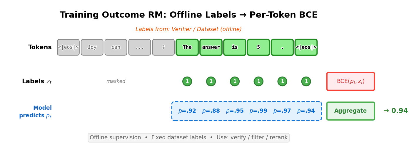
These models have continued to be used, but are less supported in open-source RLHF tools. For example, the same type of ORM was used in the seminal work Let’s Verify Step by Step [12], but without the language modeling prediction piece of the loss. Then, the final loss is a cross-entropy loss on every token, predicting whether the final answer is correct.
Given the lack of support, the term outcome reward model (ORM) has been used in multiple ways. Some literature, e.g. [11], continues to use the original definition from Cobbe et al. 2021; others use it more broadly for any verifier trained to predict whether a completion is correct.
Process Reward Models
Process Reward Models (PRMs), originally called process-supervised reward models, are reward models trained to output scores at every step in a chain-of-thought reasoning process. These differ from a standard RM that outputs a score only at an EOS token or an ORM that outputs a score at every token. Process Reward Models require supervision at the end of each reasoning step, and then are trained similarly where the tokens in the step are trained to their relevant target – the target is the step in PRMs and the entire response for ORMs.
Following [12], a binary-labeled PRM is commonly optimized with a per-step cross-entropy loss:
\[\mathcal{L}_{\text{PRM}}(\theta) = - \mathbb{E}_{(x, s) \sim \mathcal{D}} \left[ \sum_{i=1}^{K} y_{s_i} \log r_\theta(s_i \mid x, s_{< i}) + (1 - y_{s_i}) \log \left(1 - r_\theta(s_i \mid x, s_{< i})\right) \right] \] {#eq:prm_loss}
where \(s\) is a sampled chain-of-thought with \(K\) annotated steps, \(y_{s_i} \in \{0,1\}\) denotes whether the \(i\)-th step is correct, and \(r_\theta(s_i \mid x, s_{< i})\) is the PRM’s predicted probability that step \(s_i\) is valid conditioned on the original prompt \(x\) and all previous steps \(s_{< i}\).
Here’s an example of how this per-step label can be packaged in a trainer, from HuggingFace’s TRL (Transformer Reinforcement Learning) [13]:
# Get the ID of the separator token and add it to the completions
separator_ids = tokenizer.encode(step_separator, add_special_tokens=False)
completions_ids = [completion + separator_ids for completion in completions_ids]

# Create the label
labels = [[-100] * (len(completion) - 1) + [label] for completion, label in zip(completions_ids, labels)]
Traditionally PRMs are trained with a language modeling head that outputs a token only at the end of a reasoning step, e.g. at the token corresponding to a double new line or other special token. These predictions tend to be -1 for incorrect, 0 for neutral, and 1 for correct. These labels do not necessarily tie to whether or not the model is on the right path, but rather to whether the step is correct.

An example construction of a PRM is shown below.
import torch.nn as nn
import torch.nn.functional as F

class ProcessRewardModel(nn.Module):
    def __init__(self, base_lm, num_classes=3):
        super().__init__()
        self.lm = base_lm  # e.g., AutoModelForCausalLM
        self.head = nn.Linear(self.lm.config.hidden_size, num_classes)

    def forward(self, input_ids, attention_mask=None, labels=None):
        """
        The inputs are tokenized prompts and completions, where the end of a
         "reasoning step" is denoted by a designated separator token such as a
         newline or other special marker rather than batch padding.
        labels will be a list of labels, True, False, and Neutral (3 labels) which
         will be predicted by the model.
        If labels=None, this is an inference-only forward pass and the loss is
         returned as None.
        """
        outputs = self.lm(
            input_ids=input_ids,
            attention_mask=attention_mask,
            output_hidden_states=True,
            return_dict=True,
        )
        # Final hidden states: (batch, seq_len, hidden_size)
        hidden = outputs.hidden_states[-1]
        # One logit vector per token: (batch, seq_len, num_classes)
        logits = self.head(hidden)

        # Inference-only forward pass: no loss is computed.
        if labels is None:
            return None, logits
        # Only compute loss at step boundaries (where labels != -100)
        # Labels map: -1 -> 0, 0 -> 1, 1 -> 2 (class indices)
        mask = labels != -100
        loss = None
        if mask.any():
            loss = F.cross_entropy(
                logits[mask], labels[mask]
            )
        else:
            loss = logits.sum() * 0
        return loss, logits
The core loss function looks very similar to outcome reward models, with the labels being applied at different intervals.
# Assume model outputs 3-class logits per token
hidden = model.lm(**inputs, output_hidden_states=True).hidden_states[-1]
logits = model.head(hidden)  # (batch, seq_len, 3)

# 3-class labels at step boundaries only: 0=-1, 1=0, 2=1 (others masked as -100)
mask = labels != -100
loss = F.cross_entropy(logits[mask], labels[mask])
Comparing Reward Model Types (and Value Functions)
The various types of reward models covered indicate the spectrum of ways that “quality” can be measured in RLHF and other post-training methods. Below is a summary of what the models predict and how they are trained.
| Model Class | What They Predict | How They Are Trained | LM structure |
|---|---|---|---|
| Reward Models | Sequence-level quality score \(r_\theta(x, y)\) | Contrastive loss between pairwise (or N-wise) comparisons between completions | Linear head on EOS/last-token hidden state |
| Outcome Reward Models | Probability that an answer is correct per-token | Labeled outcome pairs (e.g., success/failure on verifiable domains) | Per-token binary cross-entropy head; labels repeat the outcome label |
| Process Reward Models | A reward or score for intermediate steps at end of reasoning steps | Trained using intermediate feedback or stepwise annotations (trained per token in reasoning step) | Per-token head predicting step correctness (-1, 0, 1) |
| Value Functions | The expected return given the current state | Trained via regression to each point in sequence | A scalar regression head with per-token outputs |
A few caveats on the distinctions in this table, as the boundaries between model types are not always clear cut:
- Both in preference tuning and reasoning training, the value functions often have a discount factor of 1, which makes a value function even closer to an outcome reward model, but with a different training loss.
- A process reward model can be supervised by doing rollouts from an intermediate state and collecting outcome data. This blends multiple ideas, but if the loss uses per-reasoning-step labels, it is best referred to as a PRM.
What if you train a Bradley-Terry pairwise model with correct/incorrect pairs? Much of the confusion on outcome reward models came from a small set of the literature that was training a reward model on pairwise data derived from answer correctness. In this domain, you set the chosen response as being a correct answer to a problem and a rejected response as being an incorrect answer for the same problem. This is technically not an ORM and still trained directly with the contrastive, sequence-level loss. This is technically still a Bradley-Terry model and would fall in the first class of models we covered.
ORM vs. Value Function. ORMs and value functions can appear similar since both produce per-token outputs with the same head architecture, but they differ in what they predict and where targets come from:
- ORMs predict an immediate, token-local quantity: \(p(\text{correct}_t)\) or \(r_t\). Targets come from offline labels (a verifier or dataset marking tokens/sequences as correct or incorrect).
- Value functions predict the expected remaining return: \(V(s_t) = \mathbb{E}\left[\sum_{k \geq t} \gamma^{k-t} r_k \mid s_t\right]\). Targets are typically computed from on-policy rollouts under the current policy \(\pi_\theta\), and change as the policy changes (technically, value functions can also be off-policy, but this is not established for work in language modeling).
If you define a dense token reward \(r_t = \mathbb{1}[\text{token is correct}]\) and use \(\gamma = 1\), then an ORM is learning \(r_t\) (or \(p(r_t = 1)\)) while the value head is learning the remaining-sum \(\sum_{k \geq t} r_k\). They can share the same base model and head dimensions, but the semantics and supervision pipeline differ: ORMs are trained offline from fixed labels, while value functions are trained on-policy and used to compute advantages \(A_t = \hat{R}_t - V_t\) for policy gradients.
Inference Across Reward Model Types
The models handle data differently at inference time (once they’ve been trained), in order to handle a suite of tasks that RMs are used for.
Bradley-Terry RM (Preference Model):
- Input: prompt \(x\) + candidate completion \(y\)
- Output: single scalar \(r_\theta(x, y)\) via a linear layer from the EOS/last-token hidden state
- Usage: rerank \(k\) completions, pick top-1 (best-of-N sampling); or provide terminal reward for RLHF
- Aggregation: Not needed with scalar outputs
Outcome RM:
- Input: prompt \(x\) + completion \(y\)
- Output: per-token probabilities \(p_t \approx P(\text{correct at token } t)\) over completion tokens
- Usage: score finished candidates; aggregate via mean, min (tail risk), or product \(\prod_t p_t\) (equivalently, sum log-probabilities \(\sum_t \log p_t\))
- Aggregation choices: mean correctness, minimum \(p_t\), average over last \(m\) tokens, or threshold flagging if any \(p_t < \tau\)
Process RM:
- Input: prompt \(x\) + reasoning trace with step boundaries
- Output: scores at step boundaries (e.g., class logits for correct/neutral/incorrect)
- Usage: score completed chain-of-thought; or guide search/decoding by pruning low-scoring branches
- Aggregation: over steps (not tokens) — mean step score, minimum (fail-fast), or weighted sum favoring later steps
Value Function:
- Input: prompt \(x\) + current prefix \(y_{\leq t}\) (a state)
- Output: \(V_t\) at each token position in the completion (expected remaining return from state \(t\))
- Usage: compute per-token advantages \(A_t = \hat{R}_t - V_t\) during RL training; the values at each step serve as baselines
- Aggregation: typically take \(V\) at the last generated token; interpretation differs from “probability of correctness”
In summary, the way to understand the different models is:
- RM: “How good is this whole answer?” → scalar value
- ORM: “Which parts look correct?” → per-token correctness
- PRM: “Are the reasoning steps sound?” → per-step scores
- Value: “How much reward remains from here?” → baseline for RL advantages
Generative Reward Modeling (a.k.a. LLM-as-a-judge)
With the cost of preference data, a large research area emerged to use existing language models as a judge of human preferences or in other evaluation settings [14]. The core idea is to prompt a language model with instructions on how to judge, a prompt, and two completions (much as would be done with human labelers). An example prompt, from one of the seminal works here for the chat evaluation MT-Bench [14], follows:
[System]
Please act as an impartial judge and evaluate the quality of the responses provided by two AI assistants to the user question displayed below.
You should choose the assistant that follows the user's instructions and answers the user's question better.
Your evaluation should consider factors such as the helpfulness, relevance, accuracy, depth, creativity, and level of detail of their responses.
Begin your evaluation by comparing the two responses and provide a short explanation.
Avoid any position biases and ensure that the order in which the responses were presented does not influence your decision.
Do not allow the length of the responses to influence your evaluation.
Do not favor certain names of the assistants.
Be as objective as possible.
After providing your explanation, output your final verdict by strictly following this format: "[[A]]" if assistant A is better, "[[B]]" if assistant B is better, and "[[C]]" for a tie.
[User Question]
{question}
[The Start of Assistant A's Answer]
{answer_a}
[The End of Assistant A's Answer]
[The Start of Assistant B's Answer]
{answer_b}
[The End of Assistant B's Answer]
Given the efficacy of LLM-as-a-judge for evaluation, which spawned many other evaluations such as AlpacaEval [15], Arena-Hard [16], and WildBench [17], many began using LLM-as-a-judge instead of reward models to create and use preference data.
An entire field of study has emerged around how to use so-called “Generative Reward Models” [18] [19] [20] (including models trained specifically to be effective judges [21]), but on RM evaluations they tend to be behind existing reward models, showing that reward modeling is an important technique for current RLHF.
A common trick to improve the robustness of LLM-as-a-judge workflows is to use a sampling temperature of 0 to reduce variance of ratings.
Further Reading
The academic literature for reward modeling established itself in 2024. The bulk of early progress in reward modeling has focused on establishing benchmarks and identifying behavior modes. The first RM benchmark, RewardBench, provided common infrastructure for testing reward models [22]. Since then, RM evaluation has expanded to be similar to the types of evaluations available to general post-trained models, where some evaluations test the accuracy of prediction on domains with known true answers [22] or those more similar to “vibes” performed with LLM-as-a-judge or correlations to other benchmarks [23].
Examples of new benchmarks include:
- Text-only (general chat / preferences): RMB [24], RewardBench2 [25], Preference Proxy Evaluations [26], or RM-Bench [27].
- Specialized text-only (math, etc.): multilingual reward bench (M-RewardBench) [28], RAG-RewardBench for retrieval augmented generation (RAG) [29], ReWordBench for typos [30], RewardMATH [31], or AceMath-RewardBench [32].
- Process RMs: PRM Bench [33] or ProcessBench [34] and visual benchmarks of VisualProcessBench [35] or ViLBench [36].
- Agentic RMs: Agent-RewardBench [37] or CUARewardBench [38].
- Multimodal: MJ-Bench [39], Multimodal RewardBench [40], VL RewardBench [41], or VLRMBench [42].
To understand progress on training reward models, one can reference new reward model training methods, with aspect-conditioned models [43], high-quality human datasets [44] [45], scaling experiments [46], extensive experimentation [47], or debiasing data [48].
Suggested Experiments
The companion code repository includes small reward model training scripts in code/reward_models/. These are intended as learning exercises rather than tuned reference recipes. Start from a clean code/ environment with uv sync, then run one experiment at a time.
Train a Bradley-Terry preference reward model on UltraFeedback. Run:
cd code/
uv run python -m reward_models.train_preference_rm --samples 2000 --epochs 1
Watch whether the reward margin between chosen and rejected responses grows in the demo and W&B logs. Then vary
--samples,--lr, and--model-idto see when the signal becomes noisy or unstable.Compare outcome and process supervision. Run the GSM8K outcome reward model and the PRM800K process reward model:
cd code/
uv run python -m reward_models.train_orm --samples 400 --epochs 2
uv run python -m reward_models.train_prm --samples 500 --epochs 2
Compare what each model can score after training: the ORM should distinguish correct and incorrect final answers, while the PRM should assign scores across intermediate reasoning steps. This is the practical version of the distinction between sequence-level, outcome-level, and process-level supervision.
Add a small held-out reward model eval. A useful contribution is a 50- to 200-example evaluation for
reward_models/that reports accuracy or preference-pair ordering without requiring a full training run. Keep the evaluation small enough that it can be used while tuning hyperparameters.